2DTL
Modeling 2D (TL)
The Transmission Line Modeling method
parses a single trace or a group of traces and divides them into a finite
number of straight segments. For each segment the program checks for any
conductive areas surrounding the traces which may serve as reference conductors.
All traces in a segment, in combination with additional
reference areas, define its cross-section. The primary transmission line
parameter per unit length (R’,
L’, C’, G’) will be calculated by a static
2D field solver. In a following step all segments will be transformed
into an equivalent circuit. The
procedure even considers vias and creates related equivalent circuits
as well. Finally all circuits will be connected together into one single
electrical model representing the whole trace or group of traces.
The procedure implies that only TEM
propagation modes can be considered and this causes a limitation.
The model is only valid in a frequency range from DC to a maximum frequency.
This is due to the fact that the primary transmission line parameters
are static parameters and only valid when the geometric dimensions behind
the 2D field calculation are significantly smaller than the shortest wavelength
of the propagating wave. The method is best used in the classical
SI analysis where wave propagation effects on signal lines into
high-speed multi-layer boards have to be analyzed. The method assumes
ideal power delivery systems and does not take into account any effects
like ground bouncing.
The figure below shows the dialog box for the 2DTL
solver. It consists of three separate tabs for
Selection, Meshing and
Modeling. In the upper left corner
the number of currently Selected nets
is shown. At the right hand side there is the field Length
units which allows to select a certain unit. Changing the unit
does not affect any dimensions.
Number of elements
The frame is folded by default and has to be expanded by clicking on
the +-sign first. It includes
information which is generated during the meshing
process (see 2DTL Meshing tab).
TLSections: number of straight segments
produced during the meshing process
TLSections: remaining number of straight
segments after the combination of segments with similar cross-section
Open-ended terminals: number of terminals
which do not belong to a component pin
Selection tab
The Selection
nets frame
includes all selected nets which should
be meshed and transformed into an equivalent circuit model. The nets have
to be selected in the Navigation Tree or in the Main
View. In addition, the Insert
model frame includes a list of those components (must be a passive
two-pin device, see Passive
Device Modeling) which are connected between the selected nets on
the left column. The components are found automatically and the choice
does only depend on the list of selected nets.

The toolbar above the Selected nets
frame provides buttons to select and de-select nets:
Add  : All selected nets from the Navigation
Tree will be imported and stored inside the Selected
nets frame. Any net in the list can be selected and the corresponding
information (Color, ....) will
be shown on the right hand side.
: All selected nets from the Navigation
Tree will be imported and stored inside the Selected
nets frame. Any net in the list can be selected and the corresponding
information (Color, ....) will
be shown on the right hand side.
Refresh  :
Enables the user to update the entries in the list
according to the nets which are currently selected in the Navigation
Tree. This button is necessary, because the selection of nets (i.e.
in the Navigation Tree) and their
highlighting in the Main View
does not immediately update the entries in the list. Actually the function
combines the function from button Clear
and from button Add.
:
Enables the user to update the entries in the list
according to the nets which are currently selected in the Navigation
Tree. This button is necessary, because the selection of nets (i.e.
in the Navigation Tree) and their
highlighting in the Main View
does not immediately update the entries in the list. Actually the function
combines the function from button Clear
and from button Add.
Remove  :
Removes a selected net from the list
:
Removes a selected net from the list
Clear  : Removes
all nets from the list. Afterwards the list will be empty.
: Removes
all nets from the list. Afterwards the list will be empty.
Reset  : Forces the selection in the Navigation Tree according to the items
in the list. This function corresponds to the Refresh
button, in an opposite direction: whereas the Refresh
button updates the list according to the new selected nets from
the Navigation Tree, the Reset button resets the old selection
in the Navigation Tree according
to the net items in the list.
: Forces the selection in the Navigation Tree according to the items
in the list. This function corresponds to the Refresh
button, in an opposite direction: whereas the Refresh
button updates the list according to the new selected nets from
the Navigation Tree, the Reset button resets the old selection
in the Navigation Tree according
to the net items in the list.
Pin activating
/ deactivating: A net in the Selected
nets list can be further expanded by clicking on its +-sign.
After an expansion all Component pins, that the net is connected
to, will be displayed as can be seen in the figure
below:
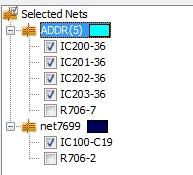
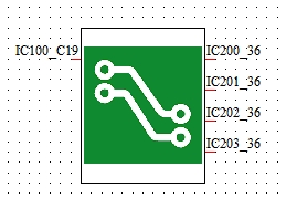
By default, those pins which are not connected to any component on
the right side are checked and every checked pin will appear in the schematic
symbol of the equivalent circuit as shown in the figure below:
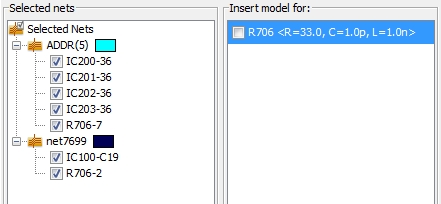
If the user wants to control the visibility of a pin he just have to
activate or de-activate the corresponding button. In the example below
the pins IC201-36 and IC203-36
are de-activated and the pin R706-7
is activated:

After another modeling step the corresponding schematic symbol will
look like in the figure below:
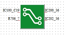
In order to activate or de-activate all pins of a certain net at once,
the user can select the corresponding net in the Select
net list, perform a right-mouse-click and choose either Include
All or Exclude All.
Insert model for:
PCBS automatically looks for passive two-pin components which are connected
between the nets listed in the Selected
nets frame. The found components are stored in the Insert
model frame on the right hand side of the dialog box. This feature
provides a convenient way to generate reasonable equivalent circuits for
a signaling path even if the path is separated in different nets. As a
prerequisite of course, an appropriate electrical model has to be assigned
to the component (see: Component Modelling).
The figure below shows a resistor (actually a resistor array) that
separates two selected nets:

By default, the components in the Insert
model frame are checked as shown in the figure below:
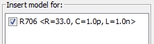
If a component is checked its equivalent circuit will be inserted within
the equivalent circuit of the overall signal path. The generated schematic
block will look like in the figure below (assumed that the corresponding
pins inside the Selected nets
frame were left unchecked):

If a component is de-activated by the user the corresponding pins in
the Selected nets frame will
be automatically activated as shown in the figure below:
The corresponding schematic block will look like in the figure below.
There are two further pins (R706_2
and R706_7) where the user can
connect a separate equivalent circuit of a resistor (see Passive
First Order Modeling):

2DTL
Meshing tab
The Meshing tab enables the
user to enter all settings which are necessary to divide the selected
nets into a group of straight segments. The figure below shows the meshing
tab:

Search distance for coupling:
Parallel segments of different (but selected) nets are considered electromagnetically
coupled if their distance is smaller than the given Search
distance for coupling. The larger this parameter is the more sections
will be coupled.
Minimum length for coupling:
Parallel segments must have a certain minimum length to be accepted
for an electromagnetic coupling. The smaller the value is the more sections
will be coupled.
Use
legacy via model:
If traces of a selected net are on different layers they are connected
by a via.
In order to account for such a discontinuity,
the program adds a corresponding via model inside
the sequence of the trace models (see Cross
section models). Two different modeling approaches for vias are available:
The legacy via model is a simple
series R/L
circuit representing the ohmic
and inductive behavior of the
vertical via tube. The advantage
is its simplicity - fewer additional circuit elements have to be added.
The disadvantage is that the approach is only accurate for frequencies
below about 1 GHz. For a higher
frequency the user is recommended to tag off the legacy
via model option. In this case, a more sophisticated kind of via
modeling technique will be used. Here, the via
model consists of a series of short modal models (see Modal
models) which were derived by a former 3D
full wave analysis and stored in an internal data
base. These via models are valid up to a frequency range of about
20 GHz.
Consider
padshapes:
From the high frequency point of view , the spot where a trace ends
in a Pad forms a discontinuity.
If the button is tagged off this discontinuity will be ignored. The advantage
is that the overall size of the model does not grow. If the button is
activated, the program internally converts the Pad
in an Area (see Areas).
As a consequence, the widening step from the trace onto the Pad
is considered and the corresponding discontinuity effect is accounted
for.
Consider
meander interaction:
In general, all conductive segments which are parallel and within the
specified Search distance
will be electromagnetically coupled during the 2DTL modeling process.
In case of a meander structure, segments of the
same nets often run in parallel and their mutual coupling can have an
erroneous impact on the delay time of the structure. If the field Consider meander interaction is de-activated
electromagnetic coupling between segments that belong to the same nets
will be not considered.
Open ended terminals frame:
This frame is folded by default and has to be expanded by clicking
on the +-sign first. It lists
all open ended terminals which
were found during the meshing process - the same open
ended terminals are searched and displayed after a PCB Layout Check. The number of open-ended
terminals is also shown inside the Number
of elements frame at the top of the dialog box. An
open ended terminal is an end
of a net which does not belong to a pin of a Component. There may
be good reason for such non-connected terminals, but they can also occur
due to a broken net which is actually not intended by the user. Therefore,
it is recommended to check this list before going ahead with the modeling
process.
Cross
sections frame:
This frame is folded by default and has to be expanded by clicking
on the +-sign first. It lists
the cross-sections of all segments which were produced during the meshing
process:
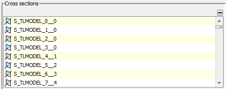
All generated segments are numbered and the corresponding number of
a specific segment appears as the first of two
numbers in the name. Segments with a similar cross-section will be combined
automatically by the program in order to save calculation time for the
2D field calculation process.
Which segments belong together is marked by the second number in the name.
In the figure above the first four cross-section belong together, because
they all have the same second number (15)
in their name. The number of all cross-sections (TLSections)
and the number of the remaining cross-sections (TLSections
after combination) are also shown inside the Number of elements frame at the top
of the dialog box.
By double-clicking on a certain
item in the list the corresponding cross-section geometry will be displayed
in a separate window as shown in the figure below. As
long as this separate window is not closed it allows the user to look
at different cross-sections by simply selecting the corresponding items
in the Cross sections list.

Start Meshing:
Starts the meshing, which means the generation of straight segments
with their corresponding cross-sections.
Show Mesh:
If this button is activated the corresponding straight segments are
highlighted in the Main View
as shown in the figure below:
View mesh text:
Displays the corresponding names to each segment as shown in the figure
below:
Hide layout:
Allows the user to hide the underlying layout geometry.
2DTL Modeling
tab
Within the Modeling tab all necessary parameters to control the
generation of an equivalent circuit can be entered and the modeling process
itself can be started.

Ohmic losses:
Decides whether the conductivity
of the conductor materials shall be taken into
account or not. If this button is activated the frequency
dependent skin-effect on the transmission lines is taken into account
(see Ohmic
loss modeling) .
Dielectric losses:
Decides whether the loss angle
of the dielectric materials shall be taken into account or not. If
this button is activated the frequency
dependent dielectric loss is taken into account on basis of a broadband Debye model
(see Dielectric
loss modeling) .
Allow modal
models:
The standard way of modeling transmission lines is to use a series
of segments consisting of so called
lumped elements, which model the primary transmission line parameters
per unit length R', L', C'. The corresponding geometric length of a single
segment is chosen by the program in such a way that its length will be
significantly smaller than the smallest wave length given by the field
Model valid up to frequency. The
shorter the segments are the better the approximation of the transmission
line effect is. The right choice of the segment length has an serious
impact on an important transmission characteristic: the phase velocity
or transmission delay. The internal rule is: a segment must have a maximum
length of 1/20th. of the smallest wave length.
If the meshing provides electrically
long segments (e.g. since the transmission lines on the PCB are not interrupted)
it is more accurate to use modal models
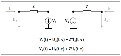
instead of lumped elements. Modal means the transmission line is not modeled
by its primary transmission line parameters but by its secondary parameters
wave impedance Z and transmission
delay t. A simple
modal model consists of two resistors on each side modeling the wave impedance
Z. In addition, there are two controlled voltage sources on both sides:
the voltage source on one side at time point "t"
is controlled by a voltage which existed at time "t-t"
on the other side of the transmission line.
There are two important advantages
of the modal model: First, the transmission
delay is an essential characteristic of the model and has not to
be approximated as is the case for the lumped
element model. Therefore, the modal
model is more accurate than the lumped
element model in any case. Second, a modal model needs only one
single segment to describe the whole transmission line, no matter how
long the transmission line actually is. Therefore, the modal model leads
to less complex models in case of electrical long transmission lines.
The disadvantage of modal models
may be an increased simulation time during a transient analysis, when
even very short segments are modeled by modal models, too. This is because
the maximum time step during a transient task must not exceed the transmission
delay of the shortest modal model (otherwise the model's delay characteristic
wouldn't be resolved.) If the button Allow
modal models is activated the program looks for segments which
equal or exceed the minimum wave length (specified by the field Model
valid up to frequency) and models them as modal models. The remaining,
electric short segments will be still modeled as lumped models.
Consider wire bond models:
Decides whether bonding wires should be considered or not. In general,
a bond wire is modeled as a simple series
R/L circuit representing
its ohmic and inductive
behavior.
Model
valid up to frequency:
Defines the frequency up to which the equivalent circuit must still
be valid. This value influences the internal size of the equivalent circuit
(the number of lumped elements and the number of additional elements due
to the modelling of ohmic and dielectric losses). Therefore, this frequency
limit should always be chosen only as high as necessary. Note: Due
to the underlying static 2D method which generates the corresponding transmission
line parameters for the segments, there is a general upper frequency limit
that couldn't be exceeded. This general limit is given on account of the
segment's cross-section dimensions which aren't allowed to exceed a certain
fraction of the wave length of the correspondent maximum frequency. If
the user's chosen maximum frequency can not be reached the program puts
out a warning in the Message
Window.
The Options
frame is folded by default. It includes some additional modeling
parameters:
Accuracy
(inside Options frame):
Controls the accuracy of the static
2D field calculation for the extraction of the transmission line
parameters. Four values are available:
normal
(default)
medium
high
very
high
Signal
type of unselected nets (inside Options frame):
If additional nets are detected within the specified
search distance they must be assigned to any of the two available types:
float
(default): Considers the net to be high ohmic floating, without any specified
voltage. This has less influence on the transmission line parameters of
the selected nets
ground:
Considers the net to be drawn at ground potential. This has more influence
on the transmission line parameters of the selected nets
Signal
type of neighbouring areas (inside Options frame):
Defines how detected areas shall be interpreted:
Approximate
signal lines as flat:
If the button is activated the height of the traces
will not be taken into account during the static 2D calculation.
The Export model frame is folded
by default. It allows the user to export the generated equivalent circuit
into a SPICE compatible sub-circuit:
Export
to file (inside Export model frame):
Specifies the directory and the file where the sub-circuit
should be written
Model
name (inside Export model frame):
Specifies the name of the sub-circuit
Simulator
(inside Export model frame):
Enables the user to select a specific SPICE format:
SPICE
2.6
SPICE
3.0
PSPICE
HSPICE
SABER
Export
Model:
This button starts the export