|
|
|
| 首页 >> CST教程 >> CST2013在线帮助系统 |
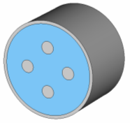
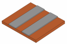
Multipin Port OverviewA multipin waveguide is characterized by having more than two conductors (e.g. two inner conductors plus shielding) in the port. According to this definition, a coplanar line is also a multipin waveguide. However, due to the importance of this particular transmission line type, it is explained in detail on the Waveguide Port Overview page.Note that the combination or superposition of different mode patterns is mostly reasonable in the case of degenerated modes. Consequently, the main application range of the multipin port operator is given by homogeneous multiple coaxial or connector ports. However, the multipin port can also be applied to inhomogeneous ports if the propagating constants of the different modes differ only slightly between each other. Please be aware that the superposition of two or more non-degenerated modes introduces inaccuracies into the transient calculation.In case of strongly inhomogeneous multi-conductor ports or pin definitions yielding to non-orthogonal mode patterns, the multipin port should be defined as a single-ended port. Then, the combination or superposition is applied to the S-parameters as a postprocessing step.Please note that the input signal of an excited waveguide port is normalized to 1 sqrt(Watt) peak power.ContentsInhomogeneous or Coupled Multipin Ports Single-Ended S-Parameter Macro Handling Multipin Waveguides by Using Standard Ports Multipin Waveguide PortsLet's first consider a simple case of a waveguide being homogeneously filled with a dielectric substrate and having more than two conductors:
The mode patterns for this type of waveguide are
frequency independent. For waveguides having N isolated conductors, (N-1)
propagating TEM type modes exist, all sharing exactly the same propagation
constant. These modes are also called degenerated
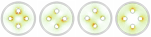
modes. The electric port mode fields for the example above are shown in
the following picture (5 conductors
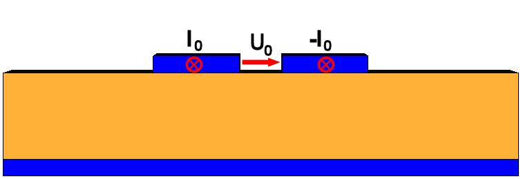
The port mode solver calculates an arbitrary superposition of the fundamental TEM modes, which unfortunately is not often the desired solution. More constraints are required to specify how to superimpose these modes to obtain the favored mode patterns. Let's now assume that you want to obtain the S-parameters for two differential pairs. Each of these differential pairs is built by two opposite conductors as shown in the following picture:
A special multipin port option allows you to specify additional constraints. An alternative approach using standard waveguide ports is explained later in the subsection Handling Multipin Waveguides by Using Standard Ports. Each of the desired excitations in the example above corresponds to a particular mode which is a superposition of the structure’s TEM modes. The necessary constraint to get the proper modes for the two pairs can be defined by assigning potential values to the conductors. The following picture shows the potential definition which yields the desired mode patterns:
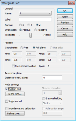
upPotential DefinitionThe definition of a multipin port starts by defining a port area of correct size (not too large and not too small) as shown in the sections above. Once the port size is determined, check the Multipin port box in the waveguide port dialog box:
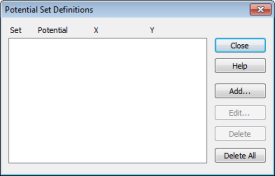
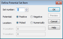
Clicking the Define Pins... button opens the following dialog box where you can assign the desired potential settings to the conductors:
A Set corresponds to a particular mode defined by assigning a certain potential distribution to the conductors. Each Set can therefore contain multiple potential definitions and represents a particular superposition of the port’s eigenmodes. In the example above, you need to define two Sets, each of which represents the mode for one of the differential pairs. To define the first conductor potential, click the Add... button to open another dialog box:
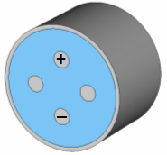
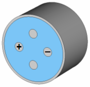
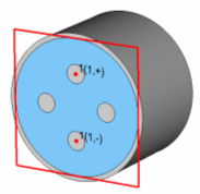
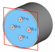
The Set Number is the first setting to make here. All Sets are simply enumerated, starting with 1. In our example, we define two Sets, named as 1 and 2. After selecting the correct set number, you can specify whether you are going to define a positive or negative potential. In this example, you need to define a positive and a negative potential for the two conductors within each pair. In most cases, it is recommended to place the potential assignment by picking the corresponding conductor in the structure view, so you can simply keep the Location being set to Picked. Clicking OK enters an interactive mode so that you can simply double-click on an end face or an edge of a conductor in order to assign the potential definition there. Once you define the two potentials for the conductors belonging to pair 1, the model should look as shown in the left picture below. After assigning the corresponding potentials to the two conductors in the second mode set (corresponding to the second differential pair), the multipin port definition is finished as visualized in the right picture:
Each of the potential definitions is labeled using the following convention: The port number is followed by a label enclosed in brackets. The first entry within the bracket gives the set number whereas the second entry depicts the type of the potential (positive or negative), e.g. ' 1(2,+) ' means: port 1, mode set 2, positive potential definition. Potential definitions on pins belonging to another potential set are set to zero. Every conductor without potential definition will be treated as a ground conductor; consequently, voltages between multiple pins with equal potential definition are set to zero. Because it is possible to select a specific pin several times for the definition of different mode sets (see section Multiple Pin Selection below), you should check that your defined potential sets are orthogonal to each other, otherwise the modes will be orthogonalized automatically by the solver to ensure a stable simulation. Taking the defined potential constraints into account, the port modes will be calculated as follows:
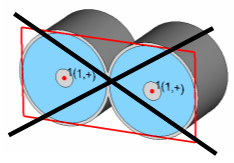
The solvers then calculate the S-parameters belonging to these mode definitions. Please note that in order to calculate the interaction of even and odd modes in a single simulation run, it is also possible to use a conductor in several mode sets at the same time. The multipin ports should not be applied to conductors that are completely shielded against each other:
For structures like this one, standard ports are preferred as shown below:
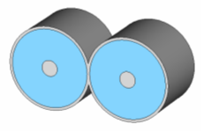
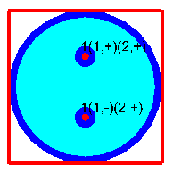
upMultiple Pin SelectionIt is possible to assign a pin conductor to more than one mode set, which lead to multiple pin selection. The following example shows the differential excitation of a double coaxial waveguide port using multiple selection of the two conductor pins:
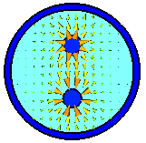
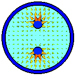
The first multipin set is defined with potential of opposite value [ 1(1,+) and 1(1,-) ], while the second modeset is determined by two positive potentials [ 1(2,+) ]. Please note that a multiple selection of conductor pins can not be used to define single-ended ports. The two resulting multipin modesets are shown by the corresponding electric field distribution. Due to the made multipin definition, both modes are orthogonal to each other.
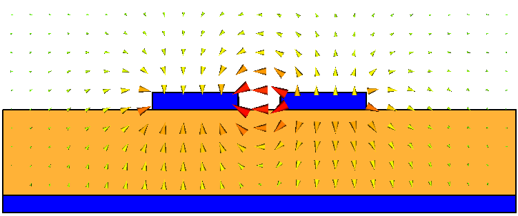
upLine Impedance DefinitionThe line impedance for multipin ports is calculated similar to the definition of a general multi conductor port as described on the waveguide port overview page by applying a formulation based on power and the sum of the currents heading into the structure. However, please note that as a difference to a general multi conductor port in case of a multipin port only those pin current values are considered which are associated to the mode set definition.
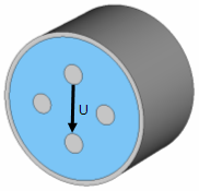
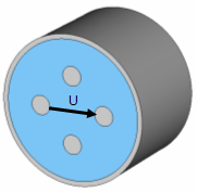
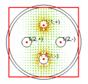
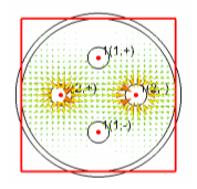
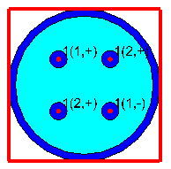
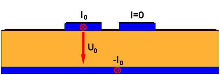
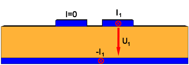
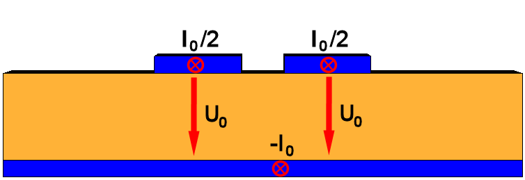
The power is given as the integral of the Poynting vector over the port area and the currents are calculated by integrating the magnetic field in a small distance around the conductors’ surfaces. Note: This impedance expression above differs from the commonly used definition Z = U / I and thus may lead to different results. See the following multipin example as a demonstration - two mode sets are defined on the four inner conductor pins of the coaxial waveguide as shown in the picture:
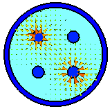
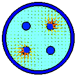
The first set is given by one positive and one negative potential value on opposite pins [ 1(1,+) and 1(1,-) ]. Set No. 2 is also defined by two potential settings, but this time both as positive values [ 1(2,+) ]. In both cases the potential belonging to the other modeset is set to zero. The resulting two mode sets are presented below, together with their corresponding line impedance value in terms of voltage U and current I :
upSymmetriesUsing symmetries in combination with multipin ports is fairly easy. If the potential definitions on both sides of the symmetry plane have the same value, one must define a magnetic symmetry due to the electric field distribution. Consequently, in case of opposite values an electric symmetry plane has to be chosen. Mode CalibrationThe mode pattern of multipin ports is orientated due to the divergence distribution of the electric field corresponding to the potential definition on the conductor pins (see examples above). The magnetic field is then determined by the power flow of the excited port, i.e., the Poynting vector of the mode pattern always points in the direction of the port radiation. upInhomogeneous or Coupled Multipin PortsFor inhomogeneous waveguides such as microstrip lines, coplanar lines, etc., the modes are generally not degenerated. In those cases, a superposition of the modes is not allowed and may lead to incorrect results. However, for relatively small frequencies or weak inhomogeneities, the modes may still be sufficiently degenerated. The solvers automatically check the level of mode degeneration and show a warning if the multipin ports should not be applied. Also in case strongly coupled multipin modes, e.g. when analyzing cross-talk behavior, it is not possible to apply a standard multipin port definition, since then orthogonal mode patterns are required. If the usage of multipin ports is not possible (for whatever reason), please see the following sections for suggestions. Single-Ended Waveguide PortsAs mentioned in case of inhomogeneous multiple-conductor ports the QTEM modes are not degenerated anymore. This means that it is not possible to create new modes as linear combinations of the existing ones. However, also in these cases the coupling between the conductors might be of interest, for example the crosstalk between conductors of multiple-conductor microstrip lines. This information can be obtained by so-called single-ended S-parameters, where the behavior of the system is described with respect to every single conductor, taking into account individual conductor to ground voltages (defined along the shortest possible voltage path) and conductor currents induced by the port modes, respectively. Not all multiple-conductor ports have to be defined as single-ended ports. It is also possible to simulate both single-ended and non single-ended ports simultaneously. However, when starting the simulation the solver uses the original port modes to calculate corresponding S-parameters, which then are recombined to single-ended S-parameters during a postprocessing step. At single-ended ports the corresponding single-ended modes can be accessed in the result tree. These single-ended results describe the coupling of one pin to the others. Furthermore, they can also be used in CST DESIGN STUDIO to obtain arbitrary common or differential S-parameters by a corresponding circuit connection. The single-ended port definition is also useful in case that non-orthogonal mode patterns are of interest. Here again it is not possible to excite these modes directly but receive their S-parameter behavior as a recombination of the simulation results with the original mode patterns.
Please note that single-ended S-parameter can only be achieved if a normalization to fixed impedances is done. If a renormalization is possible, it will be automatically applied after the simulation. For this task a complete S-matrix is necessary. If the normalize to fixed impedance option in the solver dialog is not set, then the reference impedance for all single-ended ports is chosen to be 50 Ohm. Of course it is still possible to renormalize to a new impedance as a post processing step. Even if no complete S-matrix is available, CST MICROWAVE STUDIO provides the opportunity to generate single-ended S-parameters with a subset of excitations if all port modes, that were not excited, are excluded from post processing. upSingle-Ended S-Parameter MacroAs an alternative method single-ended S-Parameters
can also be obtained as a secondary result using the macro Home:
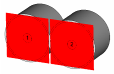
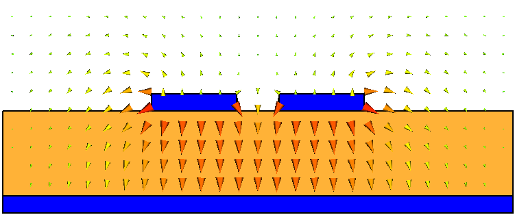
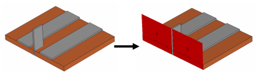
Macros Handling Multipin Waveguides by Using Standard PortsIn some cases, multiple transmission lines are located at the same side wall of the bounding box and are too close to each other to be handled as isolated transmission lines.
The preceding subsection explains the multipin port feature which provides a good solution in many cases. However, for inhomogeneous waveguides at higher frequencies, this convenient feature cannot be applied. Please note that closely neighboured transmission lines are truly physically coupled. Therefore all measurement set up will introduce some mismatch which needs to be de-embedded properly. Keep this in mind when comparing S-parameters from simulation and measurement. Disagreement is observed quite regularly when the simulation set up does not replicate the measurement set up. The easiest way to handle strongly coupled transmission line cases is to introduce a shielding at the ports in order to properly separate them. Afterward, waveguide ports can be individually applied to each of the transmission lines:
Even if this approach introduces some mismatch at the ports, of course, it may still be a viable solution. If you are unsure about the level of reflection added to the S-parameter matrix by this artificial shielding, you can simulate a short line segment alone. Ideally the reflection for the homogeneous line is zero. Therefore the actual reflection level provides some indication about the port mismatch for the particular structure. If the former approach does not produce sufficiently accurate results, the only way to handle this problem is to calculate the S-parameters for the multimode matrix by taking all propagating modes into account at each port. In transient simulations, you may also consider using the Inhomogeneous port accuracy enhancement option in the solver control dialog box to further increase the accuracy of the broadband S-parameter solution. Please refer to the Waveguide Port Overview page fore more detailed information about this feature. upSee alsoWaveguide Port Overview, Excitation Source Overview Port dialog boxes: Waveguide Port, Potential Set Definitions, Define Potential Set Item
HFSS视频教程 ADS视频教程 CST视频教程 Ansoft Designer 中文教程 |
||||||||||||||||||||||||||||||||||||||||||
|
Copyright © 2006 - 2013 微波EDA网, All Rights Reserved 业务联系:mweda@163.com |
|