|
|
|
| 首页 >> CST教程 >> CST2013在线帮助系统 |
Frequency Domain Solver OverviewWhen a time-harmonic dependence of the fields and the excitation is assumed, Maxwell's equations may be transformed into the frequency domain. The fields are then described by phasors that are related to the transient fields by multiplying the phasor with the time factor and taking the real part:
For the discretization of the geometry, the hexahedral mesh as well as the tetrahedral mesh may be chosen on demand right before the solver start. The latter is the recommended default.Different solver methods are available for the Frequency Domain solver. Among these, the General Purpose method offers the widest range of applications, and the specialized Resonant: S-Parameter methods are dedicated to the fast calculation of broadband S-parameter results.The General Purpose Frequency Domain Solver method calculates the solution for the underlying equation for a single frequency at a time, and for a number of adaptively chosen frequency samples in the course of a frequency sweep. For each frequency sample, the linear equation system will be solved by an iterative (for instance conjugate gradient) or sparse direct solver. A solution at the given frequency comprises the field distribution as well as the S-parameters and derived quantities.In case of the General Purpose method, Frequency samples can be calculated in parallel using distributed computing (besides submitting a single remote calculation, or running parameter sweeps and optimizations in parallel), see the corresponding frame in the Frequency Domain Solver Parameters and the section distributed computing and adaptive sampling below.The Resonant: Fast S-Parameter method with tetrahedral mesh calculates S-parameters as well as fields. With hexahedral mesh, the method provides S-parameters only, but no fields. The Resonant: S-Parameter, fields method should be chosen for the hexahedral mesh if, in addition to the S-parameters, field monitors are of interest.For all these solver methods it is possible to efficiently calculate electric and magnetic field monitors after an S-Parameter calculation has finished. It is not necessary to define monitors before the solver starts. See Calculate field at axis marker in the 1D-Plot Overview for further details.The fast resonant methods do not require any frequency sampling, and therefore the description hereinafter does not apply to them.Areas of application of the general purpose frequency domain solvers
Frequency sampling If you are interested in structure's S-parameters, the sampling method has a large influence on the calculation time. Automatically chosen frequency samples in conjunction with the broadband frequency sweep option usually will yield the broadband S-parameters with a minimal number of frequency solver runs. Once the S-parameter sweep has finished, the solver can continue the S-parameter sweep just where it stopped, for instance in order to calculate additional samples, monitors, and further improve the sweep accuracy. Example: A broadband frequency sweep with automatic sampling
In this example seven frequency samples are calculated in a sub interval of the global frequency range. Please note that less than twenty samples are calculated, since the S-parameter convergence criterion is reached earlier. In this case, the number of frequency samples in the Frequency Domain Solver Parameters dialog represents an upper limit. You will see a quasi continuous curve when the broadband frequency sweep has been activated. The frequency samples are shown when Additional marks is checked in the 1D plot properties dialog, which can be invoked from the context menu when viewing S-parameters. If you deactivate the sweep in the Frequency Domain Solver Parameters dialog and press Apply, the samples which actually have been calculated will be shown as well, without the intermediate values.
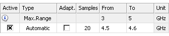
Example: A broadband frequency sweep with unlimited automatic sampling
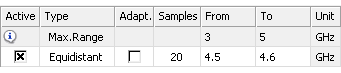
It is not necessary to define a maximum number of sample for the frequency sampling. When the number of samples is not defined (left blank) as shown above, the solver stops calculating additional samples as soon as the S-parameter sweep convergence criterion is satisfied. The results are the same as above, because the S-parameter sweep had converged after calculating seven frequency samples. Example: A broadband frequency sweep with equidistant sampling
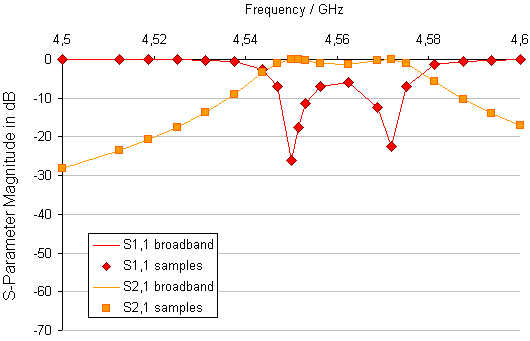
In this example twenty frequency samples are distributed equidistantly in a sub interval of the global frequency range with a frequency spacing of
You will see a quasi continuous curve when the broadband frequency sweep has been activated. The frequency samples are shown when Additional marks is checked in the 1D plot properties dialog, which can be invoked from the context menu when viewing S-parameters. If you deactivate the sweep in the Frequency Domain Solver Parameters dialog and press Apply, the samples which actually have been calculated will be shown as well, without the intermediate values.
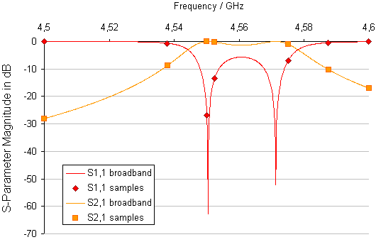
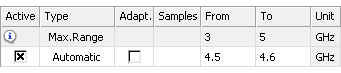
Example: Automatic sampling without broadband sweep
Here twenty samples are calculated, but obviously more samples would be required to get an accurate representation of the S-parameter poles. Please note that the broadband frequency sweep can be activated again after the simulation run in the Frequency Domain Solver Parameters dialog as a post processing step. Check the corresponding box and press Apply.
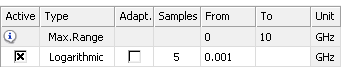
Example: Logarithmic sampling
Here five samples between 0.001 GHz and 10 GHz are calculated (the field in the column "To" is left blank, and interpreted as the upper limit of the global frequency range therefore.) With logarithmic sampling, the solver will place frequency samples at 0.001 GHz and 10 GHz, followed by 1 GHz, 0.1 GHz, and finally 0.01 GHz. If the value "From" evaluates to Zero (for instance, because the field "From" was left blank and the global frequency ranges starts at Zero), it is replaced by some suitable, arbitrary, non-zero lowest frequency automatically. Please note that you cannot enter 0 as a lower limit for logarithmic and equidistant sampling, however. Distributed computing and adaptive sampling The number and position of frequency sampling points may differ if distributed computing is enabled. This is because the adaptive sampling is no more done in a sequential manner. First of all, if the tetrahedral mesh has been chosen, all the homogeneous port modes are calculated and eventually the sequential mesh refinement runs on one computer. The general purpose solver with hexahedral mesh proceeds as mentioned hereafter, and this information applies to the tetrahedral mesh as well. The solver takes all the remaining fixed frequency samples (usually minimum and maximum or center frequency, plus frequencies where monitors are defined) and submits those jobs to the distributed computing system. This system then decides how many of those jobs can be calculated in parallel. Limitations apply due to the license, and available resources. Afterwards, if the automatic frequency sweep is enabled, the solver decides where to put the next few samples, and again submits those to the distributed computing system. As mentioned above, this can lead to a different number of samples compared to a sequential frequency sweep, that is when the solver runs on one computer. Usually the more fix points need to be calculated, the more efficient is the parallel calculation using distributed computing. Unit cells of infinite arrays Unit cell and periodic boundary conditions are used to model an infinite array consisting of a identical copies of a so called unit cell. For this unit cell, the fields for two opposite periodic boundary planes are related by a complex factor, which is determined by the phase shift. For frequency domain calculations, you may alternatively specify this phase shift by entering the constant angle of incidence corresponding to a plane wave propagating in the direction given in spherical coordinates. See the Periodic Boundary Phase Shift dialog help page for details. Please note that when unit cell boundary conditions are combined with open boundary conditions in z-direction, the open boundaries will be automatically realized by a Floquet port, which allows to excite a plane wave. See Boundary Conditions - Unit Cell and Settings for Floquet Boundaries for details. Also note that the calculation domain with periodic boundaries can be terminated either by an open boundary condition or by a waveguide port touching the periodic boundary (which has to be created explicitly, rather than by defining an open boundary as for the unit cell boundary conditions) in Frequency Domain calculations:
Usually, the iterative solver's convergence speed is higher if a periodic waveguide port is used to truncate the calculation domain. Furthermore, the periodic waveguide port can be used for the excitation of plane waves and higher order Floquet modes at the port's location. How to start the solver Before you start the solver you should make all necessary settings. See the Frequency Domain Solver Settings for details. The Frequency Domain solver can be started by
selecting Home:
Simulation
Solver logfile After the solver has finished you can view the
logfile by selecting Post Processing:
Manage Results See also Which Solver to Use, Frequency Domain Solver Parameters, Frequency Domain Solver Sampling, Frequency Domain Solver Settings, Frequency Domain Solver Overview - Resonant: Fast S-Parameter, Frequency Domain Solver Overview - Resonant: S-Parameter, fields, Frequency Domain Solver Problem Handling, Sources and Boundary Condition Problem Handling
HFSS视频教程 ADS视频教程 CST视频教程 Ansoft Designer 中文教程 |
|
Copyright © 2006 - 2013 微波EDA网, All Rights Reserved 业务联系:mweda@163.com |
|