|
|
|
| 首页 >> CST教程 >> CST2013在线帮助系统 |
Integral Equation Solver OverviewThe integral equation solver is of special interest for electrically large models. The discretization of the calculation area is reduced to the object boundaries and thus leads to a linear equation system with less unknowns than volume methods. For calculation efficiency the equation system is solved by the Multi Level Fast Multipole Method (MLFMM) for electrically large models. For the direct solver the system matrix is dense. The integral equation solver is available for plane wave excitation, discrete face ports, waveguide ports, farfield source excitation and RSD current sources. Electric and open boundaries are supported. E-field, H-Field and Farfield monitors and surface current monitors can be set in the Integral Equation Solver.OverviewAreas of application
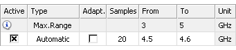
Frequency samplingIf you are interested in structure's S-parameters, the sampling method has a large influence on the calculation time. Automatically chosen frequency samples in conjunction with the broadband frequency sweep option usually will yield the broadband S-parameters with a minimal number of solver runs. Once the S-parameter sweep has finished, the solver can continue the S-parameter sweep just where it stopped, for instance in order to calculate additional samples, monitors, and further improve the sweep accuracy. Example: A broadband frequency sweep with automatic sampling
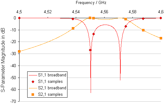
In this example seven frequency samples are calculated in a sub interval of the global frequency range. Please note that less than twenty samples are calculated, since the S-parameter convergence criterion is reached earlier. In this case, the number of frequency samples in the Integral Equation Solver Parameters dialog represents an upper limit. You will see a quasi continuous curve when the broadband frequency sweep has been activated. The frequency samples are shown when Additional marks is checked in the 1D plot properties dialog, which can be invoked from the context menu when viewing S-parameters. If you deactivate the sweep in the Integral Equation Solver Parameters dialog and press Apply, the samples which actually have been calculated will be shown as well, without the intermediate values.
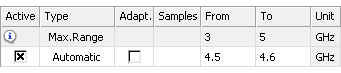
Example: A broadband frequency sweep with unlimited automatic sampling
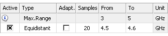
It is not necessary to define a maximum number of sample for the frequency sampling. When the number of samples is not defined (left blank) as shown above, the solver stops calculating additional samples as soon as the S-parameter sweep convergence criterion is satisfied. The results are the same as above, because the S-parameter sweep had converged after calculating seven frequency samples. Example: A broadband frequency sweep with equidistant sampling
In this example twenty frequency samples are distributed equidistantly in a sub interval of the global frequency range with a frequency spacing of
You will see a quasi continuous curve when the broadband frequency sweep has been activated. The frequency samples are shown when Additional marks is checked in the 1D plot properties dialog, which can be invoked from the context menu when viewing S-parameters. If you deactivate the sweep in the Integral Equation Solver Parameters dialog and press Apply, the samples which actually have been calculated will be shown as well, without the intermediate values.
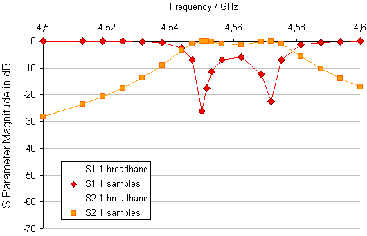
Example: Automatic sampling without broadband sweep
Here twenty samples are calculated, but obviously more samples would be required to get an accurate representation of the S-parameter poles. Please note that the broadband frequency sweep can be activated again after the simulation run in the Integral Equation Solver Parameters dialog as a post processing step. Check the corresponding box and press Apply.
Supported MaterialsA wide range of material is supported by the integral equation solver.
For material information please see also Material Parameters. How to start the solverBefore you start the solver you should make all necessary settings. See the Integral Equation Solver Settings for details. The Integral Equation solver can be started
from the Integral
Equation Solver Parameters How to create a local multilayer setup
Solver logfileAfter the solver has finished you can view the logfile
by choosing Post Processing:
Manage Results
Example for solver logfile:
Units settings: Dimensions: m Frequency: MHz Time: s -------------------------------------------------------------------------------- Boundary conditions: YZsymmetry: none XZsymmetry: none XYsymmetry: none Xmin: open Xmax: open Ymin: open Ymax: open Zmin: open Zmax: open -------------------------------------------------------------------------------- Mesh time : 68 s (= 0 h, 01 m, 08 s) -------------------------------------------------------------------------------- ================================================================================ Integral Equation Solver calculation cycle started -------------------------------------------------------------------------------- Calculation 1 of 1 (Frequency: 150 MHz) -------------------------------------------------------------------------------- The iterative solver (MLFMM) will be used. -------------------------------------------------------------------------------- Matrix setup time : 1195 s Stimulation with : Plane wave Accuracy : 0.00963581 Degrees of freedom : 92391 Iterations : 12 Solver time : 1809 s Number of surfaces : 61594 Solver order : 1st Far field memory : 1158.45 MB Near field memory : 83.5853 MB Preconditioner memory : 0.739128 MB Number of Level : [ 8 ] -------------------------------------------------------------------------------- Calculation finished. -------------------------------------------------------------------------------- Total Solver Time : 3082 s (= 0 h, 51 m, 22 s) ================================================================================
See alsoIntegral Equation Solver Parameters, Which solver to use, Multi Level Fast Multipole Method (MLFMM)
HFSS视频教程 ADS视频教程 CST视频教程 Ansoft Designer 中文教程 |
|
Copyright © 2006 - 2013 微波EDA网, All Rights Reserved 业务联系:mweda@163.com |
|