|
微波射频仿真设计 |
|
|
微波射频仿真设计 |
|
| 首页 >> Ansoft Designer >> Ansoft Designer在线帮助文档 |
|
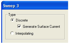
Generating Reports and Postprocessing > Overlaying Near Fields on a 3D ViewNear fields calculated as the results of a Planar EM simulation can be displayed as overlays on the 3D viewer. 1. To ensure that the near field information can be generated, the sweep setup must specify a Discrete frequency sweep, and the Generate Surface Current option must be enabled (checked):
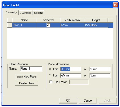
2. Run the Planar EM analysis with the sweep. 3. To display the near field overlay, expand the Analysis icon in the Project window, and select Setupm > Sweepn > Results > Near Field (m and n identify the particular solution setup and sweep setup, respectively). You can also select from a list of corresponding Setup/Sweep overlay choices which are displayed when you right-click on Field Overlays in the Project tree. 4. The Near Field dialog opens. The dialog has three tabs, described below. At the bottom of each tab are three buttons: • The Apply button is activated whenever you change a value. Click Apply to start the display, and then to see the effect of each change. The dialog stays open. • When no values were changed on any tab, the OK button starts the display. When one or more values have been changed, OK applies the changes. In either case, OK closes the dialog and adds an icon for the overlay under the Results icon in the Project window. • The Cancel button is active as long as no changes have been applied. The Cancel button closes the dialog without changing any values. If the overlay is already displayed, it does not change. If Cancel is pressed before any overlay is displayed, the overlay is cancelled. 5. The Near Field dialog opens with the Geometry tab displayed:
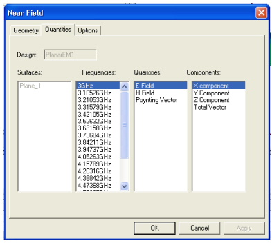
Use the options in the Geometry tab to select (or define) one or more planes for the calculation, including the dimensions to be used, and a scale factor if desired. Use the Quantities tab to select the near field quantity to be calculated:
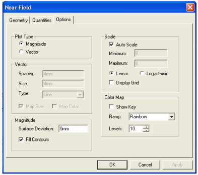
When more than one surface is involved, select a surface from the Surfaces list. Select a frequency from the Frequencies list. The frequencies are the ones swept in the analysis. Select a field type from the Quantities list. E is the electronic field, H is the magnetic field, and the Poynting Vector is the (E×H*) field, where H* is the complex conjugate of the H matrix. Select a vector component from the Components field. Use the Options tab to specify the display options for the near field overlay:
In the Plot Type panel, select Magnitude to enable the Magnitude panel options or select Vector to enable the Vector panel options. In the Scale panel, select Auto Scale (the default), or deselect Auto Scale and enter custom Minimum and Maximum scaling values. Select Linear or Logarithmic scaling (the default is Linear), and toggle Display Grid on or off (the default is off). In the Color Map panel, select the Ramp type (Rainbow is the default; other options are Hue Scale, Magenta, and Temperature), set the number of Levels (the default is 10 levels), and toggle the color key (Show Key) on and off (the default is off).
6. When you click Apply or OK in any of the Near Field dialog tabs, the 3D viewer window appears with the near field values overlaid on the geometry:
7. To dismiss the overlay, expand the Results icon in the Project window, right-click Setupm:Sweepn:Near Fieldk, and select Delete from the pulldown.
HFSS视频教程 ADS视频教程 CST视频教程 Ansoft Designer 中文教程 |
|
Copyright © 2006 - 2013 微波EDA网, All Rights Reserved 业务联系:mweda@163.com |
|