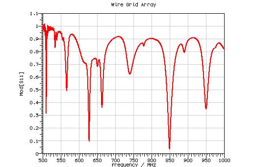
The Graph Plotter provides a view of time and frequency domain results, and near field and far field cuts.
Selecting a graph plotter will lead to the following tools in CST MICROSTRIPES becoming available.
![]() Background
color
Background
color
Change the background color between black, white and user preferred color.
![]() Open Another,
right click on plot
Open Another,
right click on plot
Load another file into the Graph Plotter to compare results. This is only possible if the X-axis units are the same for all the files. An alternative is to just drag an additional set of results from the Project View into the plot.
![]() File: Export
File: Export
Export the current view of the plot to a bitmap file. The contents of the file being viewed can be exported to a CST MICROSTRIPES format text file, or to an Excel compatible (.csv extension) file.
![]() Copy to
clipboard, CTRL-C
Copy to
clipboard, CTRL-C
Copy the view to the clipboard to allow easy pasting into a report, into another CST MICROSTRIPES plot or into a CST MICROWAVE STUDIO 1D Results folder.
![]() Options,
right click on plot
Options,
right click on plot
Opens the Graph Plotter options dialog.
![]() Grid on/off
Grid on/off
Toggle the grid display in the view.
 Linear/Log
scale
Linear/Log
scale
Toggle the scale in the Graph Plotter between Linear and Log.
In addition to displaying the data requested in the view, the Graph Plotter can also locate the maximums, minimums and zeros in the graphical data. The Locate controls are used to specify the type of feature that the user may wish to locate. This facility is available find the location of maxima, minima and zero crossings on the plot.
The user chooses whether to find the location of extrema, maxima, minima or zeros, and then clicks anywhere within the graph view. The Graph Plotter will find the nearest peak etc., and writes the value of the horizontal axis at the appropriate location. If the user chooses Locate Point, then the position of the mouse will be written onto the canvas, regardless of the plot features.
The x value, the y value, or both x and y values can be displayed on the plot, when clicking with the mouse.
If Cursor Point is turned on, then the y value of the plot nearest the cursor is dynamically displayed.
All marked positions can be cleared using Clear Markers.
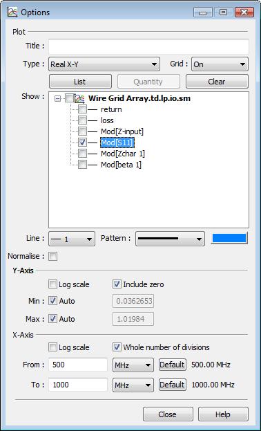
View Options are used to select which of the available output fields to plot and to control the extents of the axis.
To select items to plot the user simply identifies the required fields in the scrolling list by ticking the box next to the field.
The List and Quantity windows allows various types of real quantities to be included or excluded from the list to be plotted.
With a field highlighted by clicking on it, the color, thickness and pattern of the line used to plot the data can be changed.
The data can be plotted on X-Y coordinates or, if complex data is available, on a Smith or complex plane. If the units of the X-axis are ‘degrees’, and the X-axis has a moderate range, then polar plots become available under the Plot choice. For each coordinate system the Grid lines can be turned on or off.
The Set as reference feature can used to normalize one set of data to another. For example if a model is simulated twice, with and without a shield in position, then the results from one simulation can be normalized to the results from the second simulation to obtain the shielding effectiveness. In the plot list select an item, then click on Set as reference. Another typical use of this is to normalize results, such as E field at a point, to the input power from a port in the model.
If the items selected for plotting do not all have the same units, then a separate Y-axis is drawn for each choice of units. The range of each Y-axis may be set independently by selecting the item on the plot list and then manipulating the y axis controls.
The required Y-axis can be selected from the scrolling list and the axis limits for min and max set. These limits may be set to ‘Auto’ which allows them to vary to accommodate the range of the data or may be fixed at a particular value. For the ‘Auto’ settings, Y-max may optionally be constrained to be at least zero, and Y-min may be constrained to be not more than zero.
The extents of the X-axis can be defined by specifying the From and To values, or by using the mouse wheel to pan and zoom the plot.