

This example shows how to use the stationary thermal solver in order to compute a temperature field for an induction cooker. An induction cooker has an edge over conventional gas flame and electric cookers as it provides rapid heating and vastly improved thermal efficiency.
The setup contains a ferromagnetic coated pot and an induction coil, which creates eddy currents inside the pot. This example only focuses on the thermal properties of the structure. The main concern is with the temperature inside the induction coil which needs to be appropriately insulated in order to avoid overheating.
Most elements are created with the cylinder tool (pot, water, coil, coil-insulator) and the working coordinate system. The pot's handles are created with the torus tool and the rotate / mirror transformations. The glass plate was created with a cylinder inserted into a brick. This split-up has been done in order to create a correct surface, which carries a convection model to consider fan-cooling.
The thermal properties of most elements are taken from tables, except for the pot's bottom and the water. The pot's bottom has been set to PEC which means that it is a thermal perfect conductor. The reason for this is that the eddy currents create a thermal power of 1200 W inside the bottom which is assigned to a perfect thermal conductor. The thermal conductivity of the water-solid was set to a very high value of 1000 W/K/m in order to approximately describe the total heat-transfer through this part.
Note that in reality the heat-transfer will consist of conduction as well as convection. At the outer surfaces of the pot and the water, a convection boundary condition was applied to model the thermal loss mechanisms through these surfaces.
Except for the lower z-boundary all other boundaries are set to be of type magnetic, i.e. the normal heat flux density is zero at these boundaries. At the lower z-boundary a constant temperature is defined such that the total heat flux through this surface is zero. Due to the high dynamic of material property values it is advisable to increase the solver accuracy to 1e-9.
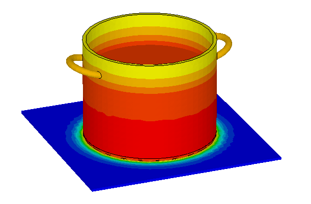
The temperature field and the heat current density can be accessed in the navigation tree under "2D/3D Results". The main interest is on the temperature inside the coil, which is approximately 60 degrees Celsius in this case. Moreover the heat flows of all source types are accessible via the "Heat Flow Values" solver-note entry.