General 1D / 0D or 1D Result from 1D Result (Rescale, Derivation, etc)

Action

Parameter

Description

Axis - scale with function f(x,y)

scale function f(x,y)

Allows you to enter a userdefined analytical function for rescaling. This function will be evaluated in the range of the chosen input signal. Function can be applied to either x- or y-axis.

Axis - scale to new range

New Minimum, New Maximum

Scales the x- or y-axis such that the minimum and the maximum fits into the given range.

Axis - Exchange x and y axes

none

Exchanges the x and the y-axis.

y - scale or shift maximum

max to 0dB / max to 1

Scales the plot such that the maximum will be 0dB or 1 respectively.

x - extract data in sub range

xlow, xhigh

Extracts the input within the range given by xlow and xhigh.

x - resample

# of Samples

resamples the whole x-range in an equidistant way

x -Upsample or Downsample

# of Samples

This option is similar to the ”x-Resample” option but it minimizes interpolation errors for equidistantly-sampled signals. When upsampling such signals, this option keeps all original samples and adds additional, linearly interpolated samples in between. This avoids, for example, cutting off peaks in the original function. When downsampling equidistantly-sampled signals, the template removes every nth sample, where n is a number that brings the number of samples after downsampling close to the number of requested samples. Please note that for this option, the resulting number of samples is usually different from the number of requested samples. It will always be larger or equal to the number of requested samples, whereas for the regular resampling option, the resulting number of samples will be identical to the number of requested samples. Although the ’r;Upsampling/Downsampling’ can be applied to inputs with non-equidistant sampling, it usually does not provide any benefits for such inputs, compared to the regular resampling. The output of ’r;Upsampling/Downsampling’ and ’r;x-Resample’ will always be sampled equidistantly.

Derivative

none

Calculates the numerical derivative

Integral

Integral kernel function

Calculates the numerical integral from with the boundaries xlow and x. Via integral kernel function, the original function can be adapted before integration step.

Time Window

Smoothness [0,100]

Applies a squared cosine windowing function to the input. The user should set the smoothness to a value from 0 to 100 to specify when the cosine shape starts. At a value of 0 the cosine window is identical to a rectangular window.

Apply Low Pass to TD/FD

Fmax

Applies a low pass filter with cutoff frequency Fmax to the original plot. There are two versions available, one simple (ideal) low pass to be applied on Frequncy Spectra, and a more sophisticated Butterworth filter, to be applied on time signals.

MC_DF (Monte Carlo Distribution Function)

none

Normalizes all x values with respect to "100*number of x values". Sorts all y values in ascending order. Then plots the normalized x over the sorted y values.

CDF (Cumulative Distribution Function)

none

Plots the cumulative distribution function.

Merge Plots

none

This option concatenates the data of the two selected plots. It is useful to add statistical data, or to stitch together two plots. The plot containing the lower x values should be selected first. This option does not perform any sorting after the concatenation and it will allow multiple y values for the same x value.

Linear Regression (first to last point)

none

Plots a straight line from the first to the last point of the original plot.

Parametric X-Y Plot

none

Takes two plots A(x) and B(x) and combines them into B(A). This can be used to create phase space plots such as Lissajous or eye patterns.
Note: This requires plot mode "Markers only".

Add Noise

Max noise amplitude

Noise Type: Uniform / 1/x

Adds noise to the signal. The noise values are equally distributed around the +- max noise amplitude and will be added per Sample.

Along the x-axis the user has the choice between uniform and 1/x decreasing noise level.

Local Averaging

N-Neighbours, Periodic

Applies a local averging in order to achieve a smoother plot. The averaging is done based on N-neighboured datapoints to EACH side.
N=0 will result in the identical, unsmoothened curve
N=1 will consider 1 datapoint above and below the original x-point -> total 3
N=2 will average between 5 data points, etc
If "Periodic" is set to 1,  the lowest  are averaged with  highest x values and vice versa, otherwise at the edges of the band neighbours are only condiered to one side.

Cross-Correlation

none

Calculates the Cross Correlation of two signals. In signal processing, cross-correlation is a measure of similarity of two waveforms as a function of a time-lag applied to one of them. This is also known as a sliding dot product or inner-product.

For signals in which the amplitude can vary, the Cross Correlation can first be normed. In this case, the Cross Correlation of two signals with identical shape will lead to a maximum correlation of 1. The position of the maximum is then the time shift between the two signal.

For numerical details please refer to: VBA-function CalculateCROSSCOR.

Cross-Correlation (normed)

none

In UWB applications, the Cross Correlation (normed) allows the user to compare the incident signal at the port (port signal) with the radiated signal (farfield probe). The position of the maximum is the runtime of the signal from port to probe.

Convolution

none

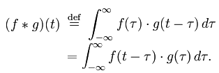
Calculates the Convolution of two signals. The convolution of  and  is written  . It is defined as the integral of the product of the two functions after one is reversed and shifted.

In electrical engineering, the convolution of one function (the input) with a brief but strong impulse (see impulse response) gives the output of a linear time-invariant system. At any given moment, the output is an accumulated effect of all the prior values of the input function, with the most recent values typically having the most influence (expressed as a multiplicative factor). The impulse response function provides that factor as a function of the elapsed time since each input value occurred.