|
|
|
| 首页 >> CST教程 >> CST2013在线帮助系统 |
Power ViewContents
1D power and loss curves
Power Accepted
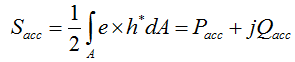
The accepted power is defined as the time average of the net power flow through the cross sectional area A of a port.
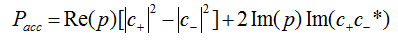
For every mode in a waveguide port or equivalently a discrete port excitation, this real power can be expressed in terms of forward (+) and backward (-) mode amplitudes c and the stimulating mode power p.
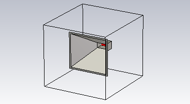
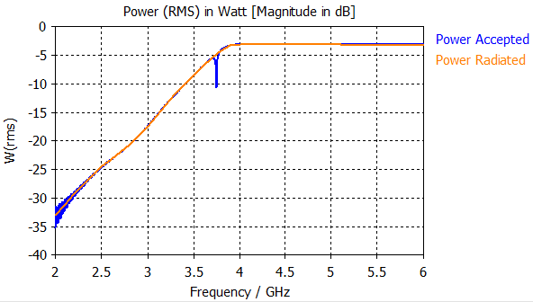
For waveguide ports considering more than one mode, the single powers per mode are added to yield the accepted power per port. (Please note that possible cross-coupling between the modes is neglected.) Finally, the real part of the sum of all accepted powers per port is shown. Example: In this example, a horn antenna surrounded by open boundary conditions is considered. The structure is excited by a rectangular waveguide port over a broad frequency range.
The power the structure accepted from the waveguide port almost completely radiates into free space.
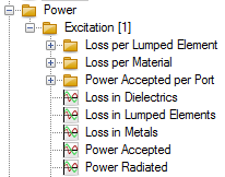
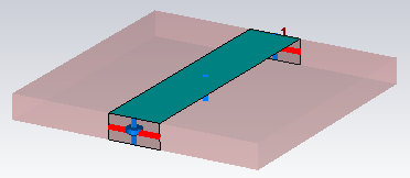
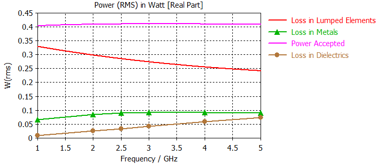
Notice that also for frequencies below the fundamental TE10 mode cut off (~3.75GHz), real net power is accepted by the antenna. Example: In this example, different loss curves are shown for a microstrip line that is modeled by a lossy metal material. Furthermore, lossy lumped and face elements are contained that accept the power inserted by port 1.
The sum of all losses equals the power accepted from port 1.
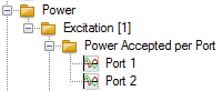
Power Accepted per Port
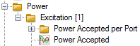
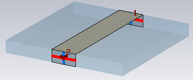
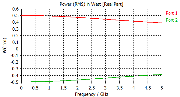
Example: In this example, a part of a microstrip line is considered. Both ends are terminated by a discrete face port. The excitation is performed via port 1.
Since there are almost no reflections in the line, the real power that could be inserted by port 1 completely leaves through port 2.Notice that for time domain calculations the energy level must have decayed sufficiently in order to obtain this result.
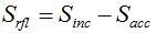
Power Reflected
The accepted power can be subtracted from the stimulated power (see below) to yield the reflected power.
It is calculated as the sum of the power that leaves the structure via all ports. Currently, only the real part of the reflected power is shown. Power Stimulated
See also 1D Result View, Post Processing Views, Navigation Tree
HFSS视频教程 ADS视频教程 CST视频教程 Ansoft Designer 中文教程 |
|
Copyright © 2006 - 2013 微波EDA网, All Rights Reserved 业务联系:mweda@163.com |
|