Background of the Simulation Method
The Finite Integration Technique (FIT)
Error Sources / Sources of Inaccuracy
Disagreement between Simulation Model and Reality
Inaccuracies due to the Simulation
CST STUDIO SUITE is a general-purpose electromagnetic simulator based on the Finite Integration Technique (FIT), first proposed by Weiland in 1976/1977 [1]. This numerical method provides a universal spatial discretization scheme applicable to various electromagnetic problems ranging from static field calculations to high frequency applications in time or frequency domain. In the following section the main aspects of this procedure are explained and extended to specialized forms concerning the different solver types.
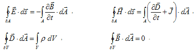
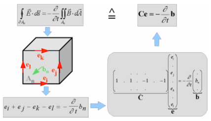
Unlike most numerical methods, FIT discretizes the following integral form of Maxwell’s equations rather than the differential one:
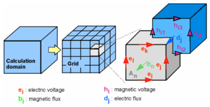
To solve these equations numerically, you must define a finite calculation domain, enclosing the considered application problem. Creating a suitable mesh system splits this domain up into many small elements, or grid cells. For simplicity, we will restrict the following explanations to orthogonal hexahedral grid systems first.
The first
or primary mesh can be visualized
in CST STUDIO SUITE in the Mesh View;
however, internally a second
or dual mesh is set up orthogonally
to the first one. The spatial discretization of Maxwell’s equations is
finally performed on these two orthogonal grid systems where the degrees
of freedom are introduced as integral values. Referring to the following
picture, the electric grid voltages e
and magnetic facet fluxes b are
allocated on the primary grid  . In addition, the dielectric facet fluxes
d as well as the magnetic grid
voltages h are defined on the
dual grid
. In addition, the dielectric facet fluxes
d as well as the magnetic grid
voltages h are defined on the
dual grid (indicated by the tilde):
Now Maxwell’s equations are formulated for each
of the cell facets separately as demonstrated in the following. Considering
Faraday’s Law, the closed integral on the equation’s left side can be
rewritten as a sum of four grid voltages without introducing any supplementary
errors. Consequently, the time derivative of the magnetic flux defined
on the enclosed primary cell facet represents the right-hand side of the
equation, as illustrated in the figure below. Repeating this procedure
for all available cell facets summarizes the calculation rule in a matrix
formulation, introducing the topological matrix  as the discrete equivalent of the analytical
curl operator:
as the discrete equivalent of the analytical
curl operator:
Applying this scheme to Ampère’s
law on the dual grid involves the definition of a corresponding dual discrete
curl operator  . Similarly the discretization of the remaining divergence equations
introduces discrete divergence operators
. Similarly the discretization of the remaining divergence equations
introduces discrete divergence operators  and
and  , belonging to the primary and dual grids,
respectively. As previously indicated, these discrete matrix operators
consist of elements ’0’, ’1’ and ’-1’, representing merely topological
information. Finally we obtain the complete discretized
set of Maxwell’s Grid Equations
(MGEs):
, belonging to the primary and dual grids,
respectively. As previously indicated, these discrete matrix operators
consist of elements ’0’, ’1’ and ’-1’, representing merely topological
information. Finally we obtain the complete discretized
set of Maxwell’s Grid Equations
(MGEs):
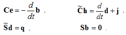
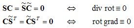
Compared to the continuous form of Maxwell’s equations, the similarity between both descriptions is obvious. Once again it should be mentioned that no discretization error has yet been introduced. A remarkable feature of FIT is that important properties of the continuous gradient, curl and divergence operators are still maintained in grid space:
At this point it should be mentioned that even the spatial discretization of a numerical algorithm could cause long-term instability. However, based on the presented fundamental relations, it can be shown that the FIT formulation is not affected by such problems since the set of MGEs maintain energy and charge conservation [2].
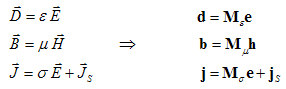
Finally, the missing material relations introduce inevitable numerical inaccuracy due to spatial discretization. In defining the necessary relations between voltages and fluxes, their integral values have to be approximated over the grid edges and cell areas, respectively. Consequently, the resulting coefficients depend on the averaged material parameters as well as on the spatial resolution of the grid and are summarized again in correspondent matrices:
Now all matrix equations are available to solve electromagnetic field problems on the discrete grid space. The fact that the topological and metric information is divided into different equations has important theoretical, numerical and algorithmic consequences [2].
In addition to orthogonal hexahedral grids, FIT can also be applied to more general mesh types such as topologically irregular grids (subgrids) and tetrahedral grids, respectively. The picture below shows the allocation of the electric voltages and magnetic fluxes on a tetrahedral mesh cell.
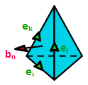
The application of FIT to these more general types of meshes can be seen as an extension to the basic method outlined above. Please refer to the references for more information [4].
In the case of Cartesian grids, the FIT formulation can be rewritten in time domain to yield standard Finite Difference Time Domain methods (FDTD). However, classical FDTD methods are limited to staircase approximations of complex boundaries. In contrast, the Perfect Boundary Approximation (PBA) technique [3] applied to the FIT algorithm maintains all the advantages of structured Cartesian grids while allowing accurate modeling of curved structures. The FI method can be even further enhanced by the Thin Sheet Technique (TST) which improves the modeling of thin perfectly electric conducting sheets.
As demonstrated, the FIT formulation is a general method and therefore can be applied to all frequency ranges from DC to high frequencies.
One outstanding feature of CST STUDIO SUITE is the Mesh on Demand strategy, which is a combination of hexahedral grids (including PBA and TST) and tetrahedral grids. This flexibility allows choosing the best-suited mesh type for every particular application. The Mesh on Demand approach is exceptionally powerful in combination with the Method on Demand capability which allows choosing the most efficient solver module for the given problem.
Currently, three electromagnetic solver products are available within CST STUDIO SUITE:
1. CST MICROWAVE STUDIO (MWS), covering the high frequency range, both in transient and in time harmonic state
2. CST EM STUDIO (EMS), the low-frequency package, which includes a variety of static and low frequency solvers
3. CST PARTICLE STUDIO (PS), the particle tracking solver package
Three solver types are available concerning high frequency electromagnetic field problems: transient, frequency domain and eigenmode solver. The purpose of the following section is to provide basic information about the solvers and to present the corresponding fundamental equations.
The CST MICROWAVE STUDIO transient solver allows the simulation of a structure’s behavior in a wide frequency range in just a single computation run. Consequently, this is an efficient solver for most driven problems, especially for devices with open boundaries or large dimensions.
The transient solver is based on the solution of the discretized set of Maxwell’s Grid Equations. Substituting the time derivatives by central differences yields explicit update formulation for the loss-free case:
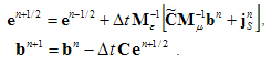
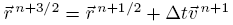
Regarding the relations above, calculation variables are given by electric voltages and magnetic fluxes. Both types of unknowns are located alternately in time, as in the well-known leap-frog scheme shown below:
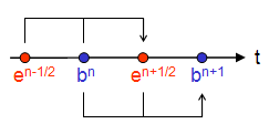
For example, the magnetic flux at t = (n+1) Dt is computed from the magnetic flux at the previous time step t = n Dt and from the electric voltage at half a time step before, at t = (n+1/2) Dt .
Explicit time integration schemes are conditionally stable. The stability limit for the time step Dt is given by the Courant-Friedrichs-Levy (CFL) criterion
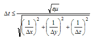
which has to be fulfilled in every single mesh cell.
The CST MICROWAVE STUDIO frequency domain solver is useful for simulating electrically small to mid-size problems or for narrowband structures. Other application areas are problems where arbitrary periodic boundaries or even unit cell boundaries are needed.
The frequency domain solver is based on Maxwell’s Grid Equations in the time harmonic case (∂ / ∂ t → iw). For loss-free problems this leads to the following second-order relation:

The general-purpose frequency domain solver can be used together with hexahedral or tetrahedral grids.
The general-purpose solver is accompanied by a solver module specialized for S-parameter calculations in highly resonant loss-free structures such as filters. This solver does not compute fields but is extremely fast compared to other simulation methods. As a third alternative, an extension of the latter solver is available which is able to calculate the fields as well. However, the additional field computation takes quite a bit of time, significantly reducing performance.
The CST MICROWAVE STUDIO eigenmode solver allows computation of the structure’s eigenmodes and the corresponding eigenvalues.
The eigenmode solver is based on the eigenvalue equation for non-driven and loss-free time harmonic problems. The solution is obtained in the loss-free case via the Krylov-Subspace or Jacobi-Davidson method:

For lossy problems, a Jacobi-Davidson solver is used.
Five different solver types are available: electrostatic, stationary current, magnetostatic, low-frequency and stationary thermal solvers. The purpose of this section is to describe the fundamental equations on which the solvers are based.
Based on the discretized Faraday’s Law without time dependency (∂ / ∂ t = 0) and the appropriate divergence equation, you can construct a linear equation system for electrostatic problems:
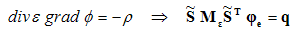
This solver module can be used together with hexahedral or tetrahedral grids.
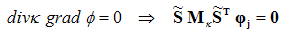
Based on the discretized Ampere’s Law without time dependency (∂ / ∂ t = 0) and the appropriate divergence equation, you can construct a linear equation system for stationary current problems:
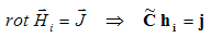
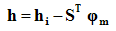
To solve magnetostatic field problems, a non-physical vector field hi is constructed in a first step fulfilling Ampère’s Law:
In general, this field contains magnetic charges that can be eliminated by solving a scalar field problem:
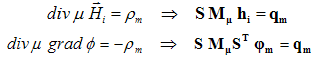
Finally, the actual magnetic field vector solution can be obtained from the hi field and the scalar potential by:
This solver module can be used together with hexahedral or tetrahedral grids.
The LF Frequency Domain solver is based on Maxwell’s Grid Equations in the time harmonic case (∂ / ∂ t → iw). It can solve three different equation types.
Fullwave
Magnetoquasistatic (MQS)
Electroquasistatic (EQS)
For the Fullwave and the MQS equation type a vector potential formulation is used:

The full Maxwell equation takes all time derivatives into account:

For the MQS equation type the displacement currents in Ampere's law are dropped. This approximation is well suited for applications where the magnetic field is dominant.

In both cases a formulation based on the magnetic vector potential is used. These equation types can be used together with hexahedral or tetrahedral grids.
For the EQS type the time derivative of the magnetic flux density is dropped in Faraday's law. This approximation is well suited for applications where the electric energy is dominant. A complex scalar potential formulation is used. For this equation type a tetrahedral based solver is available only.

CST PARTICLE STUDIO contains some of the solver modules which have been already discussed above:
Electrostatic solver
Magnetostatic solver
Eigenmode solver
In addition to this, CST PARTICLE STUDIO also includes some specialized solvers which will be explained in the following. Note that CST PARTICLE STUDIO is currently operating on hexahedral grids only.
The CST PARTICLE STUDIO Particle Tracking Solver calculates the effect of electromagnetic fields on the movement of charged particles.
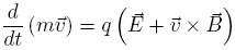
The solver is based on the discretized versions of the electric- and magnetic force law:
|
|
Analytic |
Discrete |
|
Momentum update: |
|
|
|
Position update: |
|
|
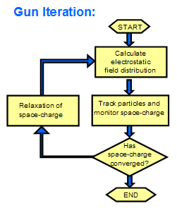
The Gun Iteration Solver performs alternately electromagnetic calculations of space charge effects and particle tracking calculations. Based on a previous particle tracking run, the corresponding electric space charge caused by the particles is calculated. Then the electric field caused by the space charge is calculated and considered for the next particle tracking iteration. This iteration is repeated until convergence is reached. The picture below illustrates this scheme:
[1] Weiland, T.: A discretization method for the solution of Maxwell's equations for six-component fields: Electronics and Communication, (AEÜ), Vol. 31, pp. 116-120, 1977.
[2] Weiland, T.: Time domain electromagnetic field computation with finite difference methods. International Journal of Numerical Modelling, Vol. 9, pp. 295-319, 1996.
[3] Krietenstein, B.; Schuhmann, R.; Thoma, P.; Weiland, T.: The Perfect Boundary Approximation technique facing the challenge of high precision field computation: Proc. of the XIX International Linear Accelerator Conference (LINAC’98), Chicago, USA,
pp. 860-862, 1998.
[4] T. Weiland: RF & Microwave Simulators - From Component to System Design Proceedings of the European Microwave Week (EUMW 2003), München, Oktober 2003, Vol. 2, pp. 591 - 596.
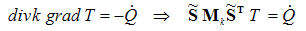
Based on the discretized Fourier’s Law of Heat Conduction without time dependency (∂ / ∂ t = 0) and the appropriate divergence equation, a linear equation system for stationary thermal problems can be derived:
Based on the discretized Fourier’s Law of Heat Conduction with time dependency.
Based on the discretized equations of balance of linear momentum without time dependency (∂ / ∂ t = 0) and the appropriate material equations, a linear equation system for stationary structural mechanics problems can be derived:
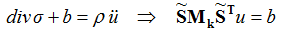
Here s represents the Cauchy stress tensor, b the external forces, r the material density and u the displacement vector.
Every discretization method is potentially affected by introducing errors either because the model is not identical to the actual device or because the numerical simulation is subject to errors itself. This section gives you an overview of the most important error sources. Many of them may be negligible in practice, but you always should be aware of them in order to make sure that you can rely on your results.
Geometric dimensions may be wrong, or geometric details may have been neglected. This happens quite often and can only be avoided by comparing the model carefully with the drawing and the real structure. The influence of small details can be studied by carrying out the same simulation with and without details.
Material parameters may be wrong either because they are not exactly known or because a value was taken which is valid for another frequency band but not for the band of interest. It might be necessary, especially when investigating a broader band, to enter the correct frequency dependency of the material values. For example, for some dielectrics a constant tan d is an appropriate choice rather than a constant conductivity.
The source of excitation may have not been chosen correctly, e.g. a perfectly matched microstrip port instead of a coax fed microstrip with normalized impedance. Furthermore, for open ports such as microstrips or coplanar lines, the port size should be chosen sufficiently large to correctly capture the field pattern of the propagating modes. Bear in mind that discrete ports are typically not perfectly matched, even when they have the same impedance as the waveguide.
The same considerations are valid for output ports for which you should try to find a simulation model that best fits the measurement structure.
Sometimes the environment is not considered correctly. Objects that are placed near the measured structure may influence the result and, in this case, should be included in the simulation model.
Discretization error: To ensure accurate results, the electromagnetic fields need to be sampled sufficiently dense in space. Generally, the accuracy of the field solution increases with a finer mesh, and it can be proven that convergence is ensured by the FI method. CST STUDIO SUITE supports convergence studies by automatic adaptation of the mesh density parameters and by visualization of the convergence progress.
Truncation error: If a transient calculation stops before the time-domain signals have decayed down to zero, a ”truncation error” is introduced.
The geometry error is the deviation between the CAD structure and the meshed model. Some methods based on orthogonal grids convert rounded structures into staircase models before starting the simulation. In tetrahedral grids, piecewise straight objects replace rounded structures. For hexahedral grids in combination with the employed PBA technique (Perfect Boundary Approximation™), the geometrical error becomes very small or even negligible, especially for rounded conductors. However, if an object becomes small compared to the size of the mesh cells, the geometry error may not always be negligible.
Some inaccuracy may be introduced by imperfect boundary conditions. In the case of radiating structures, the open space is simulated by open boundaries. For high frequency problems, the PML technique (Perfectly Matched Layer) is well suited and very accurate even when the structure is close to the object. CST STUDIO SUITE chooses the optimum size of the surrounding simulation box automatically, but in some rare cases it may be worthwhile to check the sensitivity of the result to changes of this box.
Waveguide ports have a specific open boundary technique in which the waves are decomposed into their mode patterns. This technique allows even higher accuracies than the PML boundary condition mentioned above. In cases of inhomogeneous ports such as microstrip lines, combined with very large frequency bands, it might be necessary to activate special treatment to keep the error below -50 or -60 dB. As mentioned before, the size of the waveguide port must be defined large enough.
Even if the field values are calculated correctly, interpolation errors may still occur, e.g. when deriving secondary field quantities or when calculating the field values at locations other than the grid’s edges.
Numerical errors may be caused by the finite representation of numbers but can typically be neglected for the explicit algorithm in time domain. However, except for the transient solver, a numerical error may arise when the correspondent matrix system is solved.
Taking these potential sources of inaccuracies into account, you can ensure obtaining highly accurate simulation results by performing mesh convergence studies.
Furthermore CST STUDIO SUITE offers the feature of simulating the same structure with different discretization types and solvers. This powerful option allows you to double-check the results in critical cases by even using fundamentally different mathematical approaches.